
Averaging Attacks on TableBuilder
Recently, we published our paper on arXiv, which shows two attacks on an algorithm used by the Australian Bureau of Statistics (ABS). The algorithm allows people query Australian census data through their tool called TableBuilder.
Due to the technical/mathematical nature of the paper, the attacks might be misinterpreted as highly complex or involved. This is not the case, as I shall try and explain in this blog post. Most of the mathematics in the paper is there to formally show why the attack is expected to succeed and to derive probability bounds. The attacks themselves are fairly straightforward. The first of the two attacks is just a demonstration of why it is important to apply Kerckhoffs's principle to data privacy, just as it is done in cryptography. So, I will skip this, and concentrate on the second attack; which is the main contribution of the paper.
In what follows, I will try to explain step-by-step why the algorithm behind TableBuilder (which I shall refer to as the TBE algorithm after its authors), was designed the way it is, and how it succumbs to our attack.
Unit Record vs Tabular Data
The table below shows a fake dataset which we shall use as an example. This is pretty much the same example used in our paper, except that I have now put fictitious names behind each row indicating that the data in that row belongs to that person. This representation of the dataset is what is called unit record data. However, the term "unit record data" does not seem to be well defined. For instance, the definition here agrees with how we have defined it, but the one here seems to define it as the most granular level of data (e.g., the age could be the year of birth instead of generalised to 10 year brackets as in the table). Nevertheless, we will consider any dataset presented in the form of the Fake Dataset as unit record level data, i.e., each row containing data from a single individual, since there is no limit to how granular data could be.
| Name | Suburb | Age | Gender |
|---|---|---|---|
| Jack | Redfern | 20-29 | Male |
| John | Redfern | 20-29 | Male |
| Noelia | Newtown | 30-39 | Female |
| Liz | Redfern | 20-29 | Female |
| Jimmy | Surry Hills | 40-49 | Male |
| Susan | Darlinghurst | 70-79 | Female |
When one wants to publish this data, a first step is always to remove the name column. Once that's done, the dataset looks like the one shown below. Again, each row still belongs to one individual; even though the name has been removed. So, we shall continue to call it unit record level data.
| Suburb | Age | Gender |
|---|---|---|
| Redfern | 20-29 | Male |
| Redfern | 20-29 | Male |
| Newtown | 30-39 | Female |
| Redfern | 20-29 | Female |
| Surry Hills | 40-49 | Male |
| Darlinghurst | 70-79 | Female |
Now focus on the suburb of Redfern. The table below shows another way of data representation, which we call the tabular format. Basically, it divides the dataset into parts, in our case gender and age distribution, and shows counts of people that are in each gender-age pair. Notice how you can exactly recreate the three Redfern rows in the unit record level representation, simply by copying the number of times each tuple (Redfern, Age, Gender) appears. The take away here is that even though the data is formatted as a table rather than in unit record format, it is still possible to convert the data to the latter format for sub-populations of interest (Redfern, in our case) or for the entire database (by constructing similar tables for other suburbs).
| Age | Gender | |
|---|---|---|
| Male | Female | |
| 10-19 | 0 | 0 |
| 20-29 | 2 | 1 |
| 30-39 | 0 | 0 |
| 40-49 | 0 | 0 |
| 50-59 | 0 | 0 |
| 60-69 | 0 | 0 |
| 70-79 | 0 | 0 |
Privacy
Now imagine that we wish to build a tool that allows access to this dataset (so that something useful can be learned from the data, e.g., average age of a Redfern inhabitant). But, we want the identity of the people hidden for privacy reasons. We therefore can't just build a tool which downloads the entire Fake Dataset by simply clicking a button. We would be tempted to release the Fake Dataset with No Names. But notice that even though names have been removed, most of the rows in the dataset are unique (in fact, all except the first two). This means that an attacker knowing someone's age, gender and residential location can easily attach an identity to the corresponding row of the data. Is "most rows being unique" just an artefact of this (fake) dataset? or is it true in general? It turns out that it is indeed true of real datasets with moderately large dimension (number of columns). This has been known for a long time, and I won't go into the details. Interested readers can click the link above, or many other studies demonstrating such "re-identification" attacks.
Our remaining option then is to release some sort of tabular version of the data. We can build a tool that allows the user to construct different tables from the Fake Dataset (with No Names). But we have seen that it is easy to interchange between the tabular and unit record data format. Thus, something more advanced needs to be done. For this, we consider a dataset with more rows than the Fake Dataset, whose Redfern sub-population statistics is given by table T1 below:
| Age | Gender | |
|---|---|---|
| Male | Female | |
| 10-19 | 90 | 20 |
| 20-29 | 2 | 1 |
| 30-39 | 35 | 73 |
| 40-49 | 40 | 51 |
| 50-59 | 100 | 19 |
| 60-69 | 31 | 73 |
| 70-79 | 3 | 0 |
| Age | Gender | |
|---|---|---|
| Male | Female | |
| 60-79 | 34 | 73 |
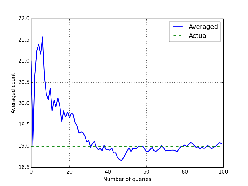
To circumvent this, another strategy is that, in addition to suppression, perturb the counts (all counts; not just low counts) by adding random noise. The analysts thus sees noisy counts and cannot carry out the differencing attack above. But notice that we can't add completely random noise, or else the output will be junk and useless for legitimate purposes. So, we can decide to add random noise within a fixed interval. Let's assume this is +/-5. Thus, instead of reporting the actual count, we would sample "fresh" noise at random, add to the count and return the noisy count as an entry in the table. The problem with this is that the analyst can create a table multiple times. If fresh noise is added to the count each time then one can launch an averaging attack. Why does it work? Notice that the noise is in the interval +/-5. Since the noise is sampled randomly each time, after a certain number of trials there will be an almost equal distribution of positives and negatives. We can add all the noisy counts, and divide it by the number of times the same table was requested to "average out" the error. An illustration of this is shown in the graph below. The analyst's target is the cell (Redfern, 50-59, Female) whose true count is 19 according to Table T1. The analyst asks the same query 100 times, and the graph shows how the average count converges to the true value. One can find the nearest integer to the fracitonal value obtained at the end (in this case 19.07) to obtain the true count.
The TBE Algorithm and Our Attack
The failure of the above techniques then led to the "same contributor, same noise" technique used in the TBE algorithm. Under this rule, if two queries (cells in a table) are satisfied by the exact same set of individuals (called contributors), then intead of adding fresh noise, the same noise will be added. This immediately renders the above-mentioned averaging attack useless. However, what we show in our paper is that there is another way to launch an averaging attack. To see this, let's assume that the perturbation parameter in TBE is +/-5. Consider Table T1 again. If we ask TBE (via the TableBuilder tool) the count of people aged 30-39 and 40-49, we would get something like this:
| Age | Gender | |
|---|---|---|
| Male | Female | |
| 30-39 | 37 | 71 |
| 40-49 | 44 | 53 |
| Total | 74 | 121 |
The first thing to note here is that the counts in each cell are noisy. The second thing is the introduction of the row titled "Total." This basically corresponds to the age range 30-49. Importantly, since the contributors in the age range 30-49 are not the same as the contributors in the age ranges 30-39 and 40-49, the noise added to the total cells is different (and hence does not add up)! Note further that this observation holds even if one of the cells 30-39 or 40-49 (under say the Female column) was suppressed (due to having a low non-zero count), since the total would include the other cell count which is not suppressed.
Now suppose that the analyst is interested in knowing the true count under (Redfern, 70-79, Male) from Table T1 with access to only the TBE algorithm. The TBE algorithm essentially suppresses this small count and returns 0. The analyst can do the following. Let M be the total number of males in Redfern (i.e., across all ages). The analyst can ask two queries: (10-19, 20-29,...,50-59) and (60-69, 70-79), receiving two tables from the TBE algorithm. Let M1 the total number of males in the age range (10-59) and let M2 denote the total number of males in the age range (60-79). Through the two tables, the analyst obtains noisy versions of these counts (through the "total" cells). Let's call them M1' and M2'. Note that M = M1 + M2. Notice also that M1 and M2 have different contributors (in fact, mutually exclusive). The analyst records the noisy sum, i.e., M1' + M2'. Let us call this N.
The analyst then chooses another "two-partition," e.g., (10-19, 20-29, ..., 40-49) and (50-59, 60-69, 70-79). Once again the sum of the number of males is equal to M. And the analyst receives noisy counts M1'' and M2''. Now, since the partitions are different, the contributors are different as well, and hence the noisy counts returned by the TBE algorithm contain fresh independent noise! The analysts adds M1'' and M2'' to the noisy sum N. Continuing on this way, the analyst obtains noisy counts for all "two-partitions". Each two-partition contains different contributors (unless the true count is 0; the analyst can discard queries whose answer under TBE is 0). For a total of m different attribute values, there are exactly such two-partitions (as shown in our paper). For our case, we have m = 7, and so 63 different two-partitions. Adding these noisy totals to N for each query, the analyst can finally divide N by the total number of two-partitions queried, and obtain the actual count M. This averaging attack works the same way as the previous simpler averaging attack except now we are carefully asking queries to ensure that we get around the "same contributors, same noise" property of the TBE algorithm.
Once the analyst has obtained M, he/she can repeat the same process to obtain the true count under M - (70-79) (by considering two-partitions without 70-79). Finally the true count of (Redfern, 70-79, Male) is obtained as the difference between the two answers. This is more or less the crux of the attack in our paper. I have excluded some technicalities (such as what to do when one of the two-partitions returns a zero count under TBE, and how many queries would ensure that the noise is removed with high confidence). These details are in our paper. For this post, notice that we can apply the same process to find the true count under each age range, and thus obtain the noiseless table for the age distribution of the entire (Redfern, Male) sub-population in the database. This table can then be converted into unit record format as explained before. Likewise, the attack can be used to "reconstruct" any target sub-population of the dataset.
Conclusion
So there it is. As you can see, the attack is fairly simple. How can the attack be mitigated? We discuss some options in our paper. However, the most sound mitigation strategy (in our opinion) is to calibrate noise according to the number of queries asked. Giving away overly accurate answers to too many queries is eventually going to violate privacy. Luckily, we do have a framework that allows us to release noisy answers to queries while simultaneously maintaining privacy. The framework is called differential privacy, proposed first in this paper. Differential privacy may not yield good utility for some use cases, however, the amount of noise added to query answers is, in many cases, close to the lower bound needed to ensure even a nominal notion of privacy. For averaging attacks, this means that the amount of noise added is such that the probability of obtaining the true count remains small (and controlled).